
You can also find all 47 answers here 👉 Devinterview.io - RNN
1. What are Recurrent Neural Networks (RNNs), and how do they differ from feedforward neural networks?
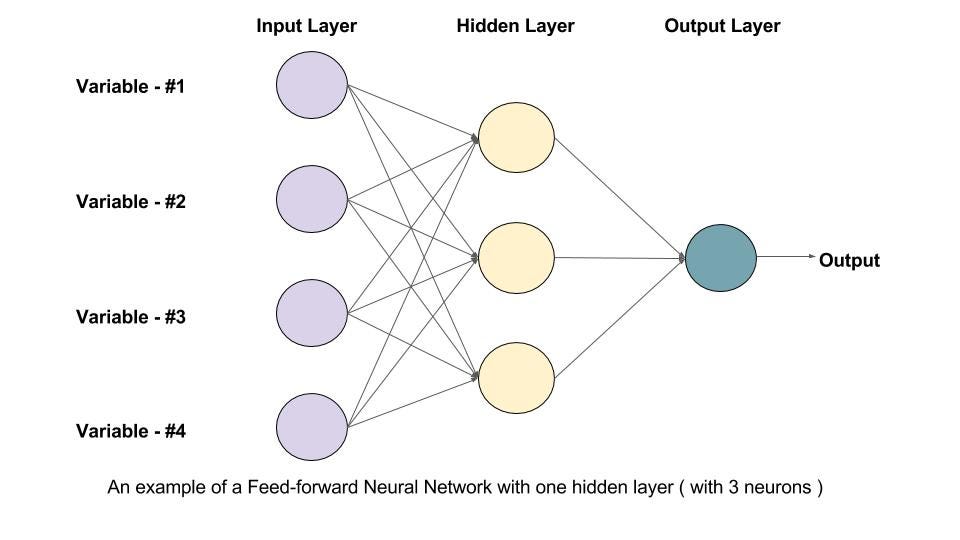
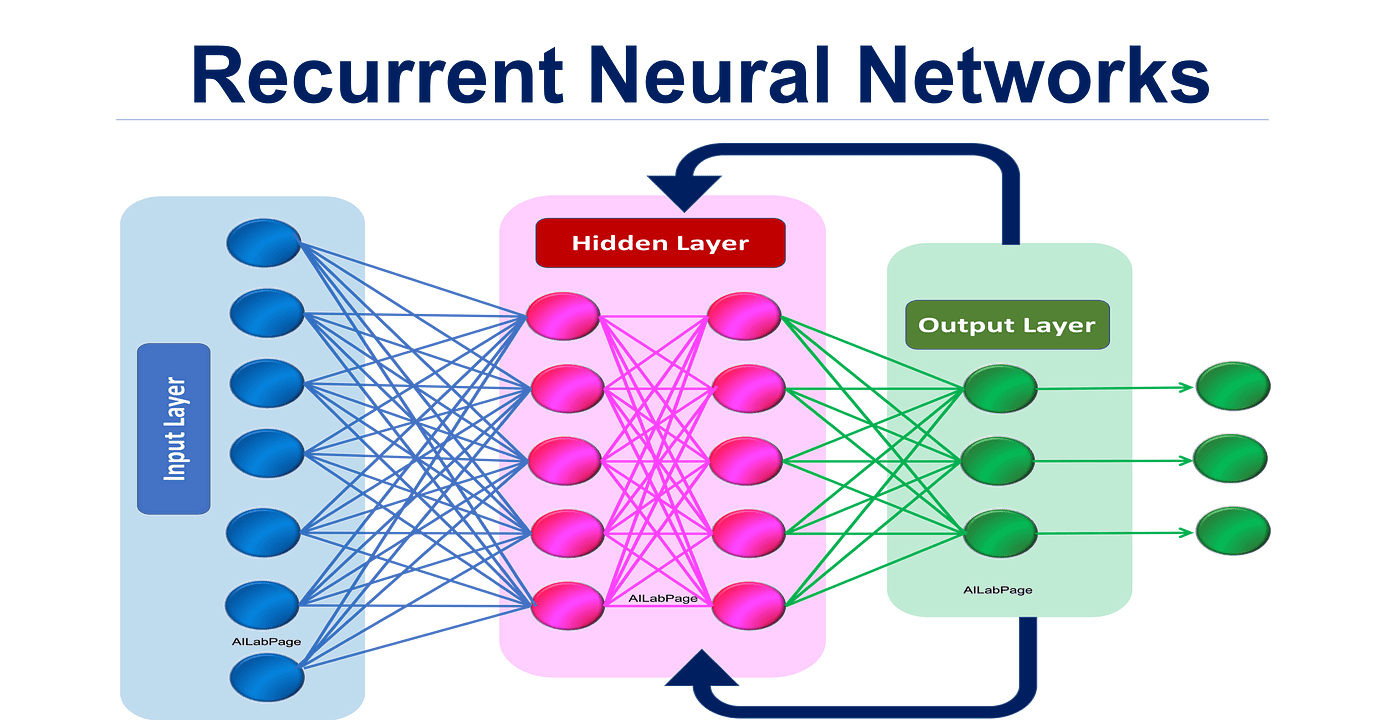
Recurrent Neural Networks (RNNs) are a specialized type of neural network specifically designed to process sequential data. Unlike traditional feedforward networks, RNNs have "memory" and can retain information about previous inputs, making them effective for tasks such as text analysis, time series prediction, and speech recognition.
-
Internal State: RNNs use a hidden state that acts as short-term memory. At each time step, this state is updated based on the current input and the previous state.
-
Shared Parameters: The same set of weights and biases are used across all time steps, simplifying the model and offering computational advantages.
-
Collapsed Outputs: For sequence-to-sequence tasks, the RNN can produce output not only at each time step but also after the entire sequence has been processed.
For sequence-to-sequence tasks, the outputs from RNNs can be combined, often using dedicated layers like an encoder followed by a decoder or using advanced architectures like LSTM and GRU.
- Feedforward Neural Networks: No inherent ability to handle sequence input.
- RNNs: Process inputs sequentially and update the hidden state at each time step.
Here is the Python code:
import numpy as np

# Define the RNN parameters
input_size = 3
hidden_size = 2

# Initialize the RNN weights and biases
W_xh = np.random.randn(hidden_size, input_size)  # Input to hidden
W_hh = np.random.randn(hidden_size, hidden_size)  # Hidden to hidden
b_h = np.random.randn(hidden_size, 1)  # Hidden bias
W_hy = np.random.randn(1, hidden_size)  # Hidden to output
b_y = np.random.randn(1, 1)  # Output bias

# Define the RNN forward pass
def rnn_forward(inputs, h_prev):
    # Compute the hidden state
    h_next = np.tanh(W_xh @ inputs + W_hh @ h_prev + b_h)
    # Compute the output
    y_pred = W_hy @ h_next + b_y
    return y_pred, h_next

# Initialize the hidden state and an input sequence
h_init = np.zeros((hidden_size, 1))
X = np.random.randn(input_size, 5)

# Perform the forward pass through time
h_t = h_init
for t in range(X.shape[1]):
    y_pred_t, h_t = rnn_forward(X[:, [t]], h_t)
    print(f"Input at time step {t}: {X[:, [t]].T}, Predicted output: {y_pred_t}")

# Example: Perform the forward pass through time
# Outputs the predicted y and the last hidden state at each time stepIn a Recurrent Neural Network (RNN), time steps represent the sequential flow of data, where each input
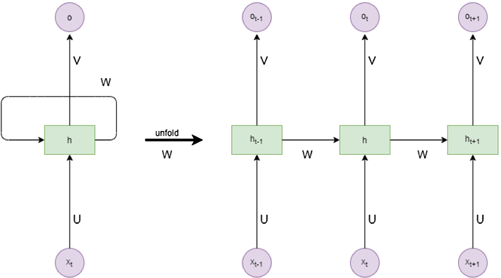
In the context of RNN Equations, the time dependence is indicated by the subscript

- Here,
$h_{t-1}$ ,$h_t$ , and$x_t$ are associated with specific time points. - The weight matrices
$W_{hh}$ and$W_{xh}$ remain constant across time steps. - On the other hand, the hidden-to-output weights
$W_{hy}$ are unique to each time step.
-
Sequence Processing: RNNs are designed to operate on sequences of data, and time steps determine the order in which sequence elements are processed. Applications like speech recognition or text generation heavily rely on this.
-
Temporal Dynamics: The presence or absence of information at a particular time influences the prediction or the hidden state at that time. This dynamic behavior makes RNNs suitable for time-series analysis.
-
Dynamic Context: The hidden state at a given time integrates all past information, making it an effective context vector for sequence tasks.
- In Unrolled RNN Diagrams, time steps are laid out horizontally, providing a visual representation of the RNN over different time points.
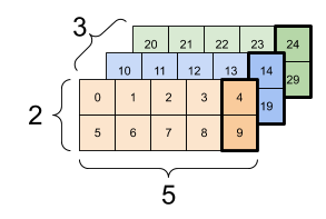
- In Tensor Shapes, data from different time steps are often shown as slices of a 3D tensor along the time dimension.
Here is the Python code:
# Importing the necessary modules
from keras.models import Sequential
from keras.layers import SimpleRNN, Dense

# Setting the number of time steps and features
time_steps = 10
features = 5

# Building the RNN model
model = Sequential()
model.add(SimpleRNN(3, input_shape=(time_steps, features), return_sequences=True))
model.add(Dense(1))
model.summary()Recurrent Neural Networks (RNN) excel in capturing long-term dependencies in both continuous and discrete-time sequences.
-
Natural Language: RNNs have widespread adoption in tasks like language modeling for text prediction and machine translation.
-
Speech Recognition: Their ability to process sequential data makes RNNs valuable in transforming audio input into textual information.
-
Time Series Data: For tasks like financial analysis and weather forecasting, RNNs are effective in uncovering patterns over time.
-
Audio Processing: In real-time, RNNs can classify, recognize, and even generate audio signals.
-
Video Processing: RNNs play a pivotal role in tasks requiring temporal understanding in videos, such as video captioning and action recognition. An example of such RNN is LSTM (Long Short Term Memory) and GRU (Gated Recurrent Unit). These are an extension of the simple RNN and efficiently model large-scale, real-world temporal dependencies.
-
3D Motion Capture: RNNs can recognize and predict human motions from a sequence of 3D positions.
-
Text-Associated Metadata: When processing documents with metadata, such as creation or modification times, RNNs can seamlessly integrate both sequences for a comprehensive understanding.
-
Multilingual Time-Series Data: In environments where languages change over time, RNNs equipped with sophisticated attention mechanisms can handle multi-lingual, time-sensitive tasks.
-
Spoken Language and Facial Expressions: For integrated understanding in tasks like understanding emotions from voice and facial expressions, RNNs provide a unified framework.
4. Can you describe how the hidden state in an RNN operates?
The hidden state in a Recurrent Neural Network (RNN) is a crucial concept that enables the network to remember previous information and use it while processing new data. It serves as the network's memory.
Role of the Hidden State
The network learns to map sequences of inputs to sequences of outputs by employing the hidden state to capture temporal dependencies or the 'context' from past information. With each new input, the RNN updates the hidden state, which retains information from all previous inputs.
where
-
$h_t$ is the hidden state at time step$t$ , -
$x_t$ is the input at time step$t$ , -
$h_{t-1}$ is the hidden state from the previous time step, and -
$f$ is a function that combines the input and previous hidden state.
At the start of the sequence, or following a 'reset,' the hidden state is typically initialized as a vector of zeros.
The calculation of the hidden state is done through the RNN activation function, often a hyperbolic tangent (
TanH:
ReLU:
where
-
$W_{hh}$ and$W_{xh}$ are weight matrices, -
$b_h$ is the bias term for the hidden state, and -
$\tanh$ or$\text{ReLU}$ are the activation functions applied element-wise.
For each step in the sequence:
-
Input-Previous Hidden State Interaction: The current input,
$x_t$ , is combined with the previous hidden state,$h_{t-1}$ , often through a matrix multiplication. -
ActivationFunction Application: The result from step 1 is passed through an activation function like
$\tanh$ or$\text{ReLU}$ . -
State Update and Output: The output becomes the hidden state at time
$t$ ,$h_t$ , and this output is also used in the next iteration as the previous hidden state, based on the representation we previously discussed.
In multilayer RNNs, each layer has its own hidden state. The output from one layer becomes the input to the next layer. The fully-connected nature of RNNs means that you can have depth not only across time steps, but also across layers. This allows the network to learn different levels of temporal features, similar to the multilayer perceptron's ability to learn distinct levels of abstraction in traditional feedforward networks.
Code Example: Hidden State Calculation
Here is the Python code:
import numpy as np

# Input data
x_t = np.array([0.2, 0.4, 0.6])
h_t_1 = np.array([0.5, 0.3, 0.8])

# Weights and biases
W_hh = np.random.rand(3, 3)  # Example only, initialized randomly
W_xh = np.random.rand(3, 3)  # Example only, initialized randomly
b_h = np.random.rand(3)  # Example only, initialized randomly

# Calculate hidden state with TanH
h_t_tanh = np.tanh(np.dot(W_hh, h_t_1) + np.dot(W_xh, x_t) + b_h)

# Calculate hidden state with ReLU
h_t_relu = np.maximum(0, np.dot(W_hh, h_t_1) + np.dot(W_xh, x_t) + b_h)While Recurrent Neural Networks (RNNs) are powerful and versatile models for processing sequential data, they are known to face several challenges when it comes to training.
Due to the multi-step backpropagation process, RNNs can suffer from vanishing (the gradient gets smaller and smaller as it's propagated back through time) and exploding (the gradient grows rapidly) gradients.
Earlier time steps are more heavily impacted in the case of vanishing gradients, and it becomes difficult for the network to effectively learn from long sequences.
RNNs have difficulty capturing dependencies between distant time steps. As a result, information can be lost or corrupted during training and make it harder for the model to learn long-range dependencies.
RNNs have a tendency to update long-term weights less often than short-term weights, which can lead to inefficiencies in training and the model's ability to process sequential data.
These issues can sometimes make it challenging for RNNs to capture the full context of a given sequence and might limit their use in certain scenarios, especially those involving lengthy or complex sequential patterns.
While RNNs are primarily associated with tasks involving sequential data, their utility is largely determined by the choice of activation function. The activation functions in RNN can be of two types: pointwise type and pointwise and temporal type.
-
Pointwise: These activations, such as ReLU, operate independently on each element of the input sequence.
-
Temporal: These functions, including tanh, are computed across time, considering the interactions and sequences.
Pointwise operations assess each input element in isolation, overlooking temporal dependencies. While this aids in computational efficiency, it may restrict the model's understanding of sequences, especially when long-term dependencies are in play.
Temporal activations, by contrast, take into account the sequence nature of the data, enabling the neural network to better capture time-evolving patterns. They can be more effective when intricate relationships and dependencies span several time steps.
The choice of an activation function also dictates how RNNs address the challenge of "vanishing" and "exploding gradients":
-
Vanishing Gradient: When gradients approach
$0$ , the RNN's learning capability diminishes early in the sequence, injuring long-term dependance modeling. The tanh and sigmoid functions can make this occurrence more probable due to their limited gradient scopes and might result in rapid saturation and weak signal propagation. -
Exploding Gradient: Conversely, if gradients become exceedingly large, the model becomes unstable, undermining the learning process. ReLUs, being unbounded and with a constant gradient, can exacerbate numerical instability and inconsistency in training.
RNNs should be able to both retain and modify information over time, a feature often referred to as "memory." Activation functions profoundly influence this capability:
-
Functions with a non-linear portion, such as sigmoid, can regulate the flow of information, effectively implementing a gate that can remember or forget data.
-
The tanh function is advantageous for RNNs: it provides a stronger gradient than the sigmoid and has a range that includes both positive and negative values, making it suitable for preserving context and preventing saturation.
While traditional activation functions like sigmoid, tanh, and ReLU play a foundational role in RNNs, newer variants such as LSTM and GRU have been developed to address some of their limitations.
For instance, LSTM relies on more intricate gates, such as the "forget gate," to mitigate vanishing gradients and bolster memory retention. This enhanced memory management typically results in more reliable long-term modeling.
Similarly, GRU is designed to be more computationally efficient by compressing the structure of the LSTM, accomplishing similar performance with fewer parameters.
Backpropagation Through Time (BPTT) is a modified version of the classic backpropagation algorithm, tailored for recurrent neural networks (RNNs).
The fundamental concept is that errors in a neural network are propagated backward through time, enabling networks like RNNs to learn sequences and time-dependent relationships.
-
Compute Output Error: Generate the error signal for the output layer by comparing the predicted output with the true target using a loss function.
-
Backpropagate the Error in Time: Starting from the output layer, propagate the error back through each time step of the RNN.
-
Update Weights: Use the accumulated errors to update the weights in the RNN.
-
Gradient Explosion: When the gradient grows too large, BPTT may become unstable.
-
Gradient Vanishing: The opposite problem, where the gradient becomes very small and difficult to learn from, especially in longer sequences.
Both these challenges are particularly pronounced in RNNs and can make learning non-trivial temporal dependencies difficult.
-
Gradient Clipping: To prevent the gradient from becoming too large, researchers often use gradient clipping, which limits the gradient to a predefined range.
-
Initialization Techniques: Using advanced weight initializers, such as the Xavier initializer, can help mitigate the vanishing/exploding gradient problem.
-
ReLU and Its Variants: Activation functions like Rectified Linear Units (ReLU) tend to perform better than older ones like the logistic sigmoid, especially in avoiding the vanishing gradient problem.
-
Gate Mechanisms in LSTMs and GRUs: Modern RNN variants, like Long Short-Term Memory (LSTM) and Gated Recurrent Unit (GRU), are equipped with gating mechanisms to better control the flow of information, making them more resistant to the vanishing gradient problem.
While Backpropagation Through Time (BPTT) is a foundational tool in training Recurrent Neural Networks (RNNs), it's not without some drawbacks.
-
Long-Term Dependencies: Unrolling over extended sequences can lead to vanishing and exploding gradients, making it hard for BPTT to capture long-range dependencies.
-
High Memory and Computation Requirements: The need to store an entire sequence and the associated backpropagation steps can be memory-intensive and computationally expensive.
-
Difficulty in Parallelization: Dependencies between time steps limit straightforward parallelization in modern hardware setups.
LSTM (Long Short-Term Memory) networks and GRUs (Gated Recurrent Units) are specialized RNN variants designed to combat many of these limitations.
Additionally, advanced techniques like truncated backpropagation through time and teacher forcing can help balance computational and memory costs while improving training efficiency. These go hand in hand with sequence-to-sequence learning.
Here is the Python code:
import tensorflow as tf
from tensorflow.keras.models import Sequential
from tensorflow.keras.layers import Embedding, LSTM, Dense
from tensorflow.keras.optimizers import Adam
import numpy as np

# Generate some sample data
data_size = 1000
max_sequence_length = 20
vocab_size = 1000

input_data = np.random.randint(1, vocab_size, size=(data_size, max_sequence_length))
output_data = np.zeros((data_size, max_sequence_length, 1))

for i, sequence in enumerate(input_data):
    for j in range(1, len(sequence)):
        output_data[i, j, 0] = sequence[j-1]

# Define and compile the model
model = Sequential([
    Embedding(input_dim=vocab_size, output_dim=64, input_length=max_sequence_length),
    LSTM(256, return_sequences=True),
    Dense(1, activation='softmax')
])

model.compile(optimizer=Adam(learning_rate=0.001), loss='sparse_categorical_crossentropy')

# Train the model using teacher forcing
epochs = 10
batch_size = 32
model.fit(input_data, output_data, epochs=epochs, batch_size=batch_size)The vanishing gradient problem identifies a key limitation in RNNs: their struggle to efficiently propagate back complex temporal dependencies over extended time windows. As a result, earlier input sequences don't exhibit as much influence on the network's parameters, hampering long-term learning.
As the RNN performs backpropagation through time (BPTT) and gradients are successively multiplied at each time step during training, the gradients can become extremely small, effectively "vanishing".
Alternatively, these gradients may explode when they get very large.
This phenomenon uniquely hinders prediction accuracy and the ability of the model to anticipate future states, especially when the training data features extended time dependencies.
- Long-Term Dependency: The network will have more difficulty "remembering" or incorporating information from the distant past.
- Inaccurate Training: Ascribed importance to historical data might be skewed, leading to suboptimal decision-making.
- Predictive Powers Compromised: The model's predictive performance degrades over extended time frames.
Unlike traditional RNNs, both Long Short-Term Memory (LSTM) and Gated Recurrent Unit (GRU) architectures proactively tackle the vanishing gradient predicament through the use of more intricate structures like gates and memory cells.
- These memory mechanisms are better equipped to capture lengthy relationships in sequential data.
- By choosing when and what information to retain, RNNs with these structures excel in tasks demanding prolonged temporal awareness.
Many modern deep learning libraries including TensorFlow, Keras, and PyTorch incorporate these advanced RNN variants. This makes them accessible not just to machine learning experts, but also to developers or researchers exploring the potential of recurrent models for a diverse range of tasks.
The vanishing gradient problem and the exploding gradient problem can both hinder the training of Recurrent Neural Networks (RNNs). However, the exploding gradient's effects are more immediate and can lead to models becoming unstable.
The exploding gradient issue arises with long-term dependencies. During backpropagation, for each time step, the gradient can either become extremely small (vanishing) or grow substantially larger than 1 (exploding).
Because RNNs involve repeated matrix multiplications, this can cause the gradient to grow (or decay) at each time step, potentially resulting in an exponentially growing gradient or a vanishing one, depending on the matrix properties.
-
Training Instability: Exploding gradients can make the learning process highly erratic and unstable. The model might converge to suboptimal solutions or fail to converge altogether.
-
Weight Updates Magnitude: Tensed weights (especially large weights) can lead to quicker or more extensive updates, making it harder for the model to find optimal solutions.
Here is the Python code:
import numpy as np

# Set random seed for reproducibility
np.random.seed(0)

# Random matrix with elements guaranteed to be larger than 1
rnn_matrix = np.random.rand(3, 3) * 2

# Initialize gradient
gradient = np.array([[2, 0, 1]])

# Perform matrix multiplication over 10 time steps
for i in range(10):
    gradient = np.dot(gradient, rnn_matrix)
    print(f"Gradient after step {i+1}:\n{gradient}")

# You can observe that the magnitude of the gradient grows rapidly-
Weight Initialization: Use techniques like Xavier or He initialization to prevent weights from starting at extremes that could exacerbate the issue.
-
Gradient Clipping: Limit the magnitude of the gradient to a threshold, e.g., 1.0, to mitigate the instabilities arising from excessively large updates.
-
Architectural Modifications:
- Gated Architectures: Models like LSTMs and GRUs are designed to mitigate the vanishing/exploding gradient problems.
- Layer Normalization: Normalize the inputs to each recurrent unit, helping to stabilize training.
- Recurrent Dropout: Applying dropout to the recurrent connections can help reduce overfitting and stabilize learning.
-
Learning Rate Schedules: Adjust the learning rate during training to help manage gradient magnitudes.
11. What are Long Short-Term Memory (LSTM) networks, and how do they address the vanishing gradient problem?
While Recurrent Neural Networks (RNNs) are powerful for handling sequential data, they can suffer from the vanishing gradient problem, where gradients can diminish to zero or explode during training.
This is a challenge when processing long sequences, as early inputs can have a pronounced impact while later inputs may be overlooked due to vanishing gradients. Long Short-Term Memory (LSTM) networks were specifically designed to address this issue.
- LSTM: Core to its design, the memory cell provides a persistent memory state. Through "gates," this state can be regulated and signals can either be forgotten or stored.
- RNN: Limited memory, as the context is a function of a sequence of inputs at the current time step and does not persist beyond this step.
- LSTM: Employs three gates, with sigmoid activation functions to regulate the flow of information: a forget gate, an input gate, and an output gate.
- RNN: Forgets the previous hidden state with each new input, as it computes a new hidden state based on the input at the current time step.
- LSTM: Uses identity () function in the information flow, relayed through the memory cell, thus mitigating the vanishing gradient issue.
- RNN: Experiences more pronounced vanishing and/or exploding of gradients due to recurring self-loops with non-linear activation functions (e.g., tanh or sigmoid).
Role of Output and Hidden States
- LSTM: Separates the memory content and information to output using the gates, producing an updated hidden state and memory cell for the next time step.
- RNN: Does not segregate the content and output, directly using the hidden state from the current step as the output for the context.
- LSTM: Better suited for processing long sequences by maintaining and selectively updating the memory cell and gating the flow of information.
- LSTM: Tends to converge faster and can be trained on longer sequences more effectively due to the mitigated vanishing gradient issue.
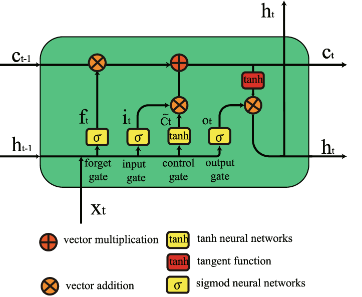
-
Memory Cell: Acts as the long-term memory component.
-
Gates:
- Forget Gate: Decides what to remove from the cell state.
- Input Gate: Modifies the cell state based on new input.
- Output Gate: Controls what to output based on cell state.
-
Candidate Values: Calculated through the tanh activation that represents potential new memory.
-
Hidden State: Represent the short-term memory or output of the LSTM cell.
-
Forget Gate:
$f_t = \sigma(W_f \cdot [h_{t-1}, x_t] + b_f)$ -
Input Gate:
$i_t = \sigma(W_i \cdot [h_{t-1}, x_t] + b_i)$ -
Candidate Value:
-
Output Gate:
$o_t = \sigma(W_o \cdot [h_{t-1}, x_t] + b_o)$ and$h_t = o_t \odot \tanh(C_t)$

Here is the Python code:
from keras.models import Sequential
from keras.layers import LSTM, Dense

model = Sequential()
model.add(LSTM(100, input_shape=(X.shape[1], X.shape[2])))
model.add(Dense(1))
model.compile(loss='mean_squared_error', optimizer='adam')
model.fit(train_X, train_y, epochs=100, batch_size=64, validation_data=(val_X, val_y), shuffle=False)Gating mechanisms in LSTM cells enable the model to remember or forget specific information over time. They've been the game-changer that made LSTMs more effective than vanilla recurrent neural networks (RNNs).
Four main gates operate within an LSTM cell, employing various sigmoid and element-wise multiplication operations:
-
Determines how much of the new information should be added to the cell state.
-
Controlled by the sigmoid function, resulting in values between 0 and 1.
-
A value of 0 means to ignore the new information, while 1 means to fully incorporate it into the cell state.
Mathematical Formula:
$$i_t = \sigma(W_i[h_{t-1}, x_t] + b_i)$$ $i_t$ : Input gate value at time$t$
$W_i$ : Weight matrix for the input gate
$x_t$ : Input at time$t$
-
Determines what information to remove from the cell state.
-
Ranges from 0 (completely forget) to 1 (completely keep).
Mathematical Formula:
$$f_t = \sigma(W_f[h_{t-1}, x_t] + b_f)$$ $f_t$ : Forget gate value at time$t$
$W_f$ : Weight matrix for the forget gate
$x_t$ : Input at time$t$
-
Controls which parts of the cell state are output as the final hidden state.
-
Modifies the cell state via a
tanhactivation function, limiting the values between -1 and 1. -
The output is then multiplied by the output gate's value.
Mathematical Formula:
$$o_t = \sigma(W_o[h_{t-1}, x_t] + b_o)$$ $o_t$ : Output gate value at time$t$
$W_o$ : Weight matrix for the output gate
$x_t$ : Input at time$t$
- The new cell state is computed by taking a weighted sum of the previous cell state and the new input.

Here is the Python code:
import numpy as np

# Sigmoid function
sigmoid = lambda x: 1 / (1 + np.exp(-x))

# Hyperparameters
hidden_size = 3
input_size = 2

# Random input and weights
x_t = np.random.rand(input_size)
h_t_prev = np.random.rand(hidden_size)
W_i = np.random.rand(hidden_size, input_size + hidden_size)
W_f = np.random.rand(hidden_size, input_size + hidden_size)
W_o = np.random.rand(hidden_size, input_size + hidden_size)
b_i = np.random.rand(hidden_size)
b_f = np.random.rand(hidden_size)
b_o = np.random.rand(hidden_size)

# Compute gates
i_t = sigmoid(np.dot(W_i, np.concatenate((h_t_prev, x_t))) + b_i)
f_t = sigmoid(np.dot(W_f, np.concatenate((h_t_prev, x_t))) + b_f)
o_t = sigmoid(np.dot(W_o, np.concatenate((h_t_prev, x_t))) + b_o)

# Compute new cell state
new_cell_state = f_t * cell_state + i_t * np.tanh(cell_input)Both LSTM and GRU networks are designed to address the issue of vanishing gradients in basic RNNs, but they do so through distinct architectures and mechanisms.
-
LSTM: Consists of a cell, input gate, forget gate, and output gate. Each component has its own set of weights.
-
GRU: Merges the cell and gate units into "update" and "reset" gates, making it computationally less intensive than an LSTM.
LSTM:

GRU:

LSTM: Employs explicit "forget" (controlled by
GRU: Uses a "reset" gate (controlled by
Recurrent Neural Networks (RNNs) and Attention Mechanisms have transformed the landscape of sequential data analysis, offering superior performance compared to traditional sequence models.
- Vanishing or Exploding Gradients: They struggle to learn from long sequences.
-
One-Size-Fits-All Representation: They treat every input step,
$x_t$ , equally.
- Dynamic Weighting: Instead of averaging all hidden states, attention sharpens the focus on pertinent ones.
- Sequence Ordering Preservation: It maintains the input's original sequence, crucial in tasks like translation.
- Visual Analogy: Think of an RNN without attention as a video played in real-time, and with attention as a tracker overlay that detects key visual elements.
- Granularity Levels: You can implement attention at various levels, ranging from individual words to segments or the entire input sequence.
- Soft vs. Hard Attention: Soft attention computes a weighted combination, while hard attention selects a single input.
- Establish the importance of each input step,
$x_t$ , via a compatibility metric, typically a neural network layer with a trained set of parameters. - Use this metric, often represented as a scalar score, in conjunction with the model's internal state,
$h_{t-1}$ , to compute a "relevance score."
- Apply a softmax function to standardize relevance scores across all time steps.
- The result is a set of weights, one for each input element, summing to 1 and facilitating weighted summation.

- Multiply the
$x_t$ sequence with their corresponding attention weight to obtain a context vector that focuses on the most important components.

- Combine the context vector with
$h_{t-1}$ to update the state, which in turn feeds into subsequent time steps or the output layer.
Here is the Python code:
import tensorflow as tf

# Create an RNN model
rnn_layer = tf.keras.layers.SimpleRNN(4, return_sequences=True, return_state=True)

# Get model outputs and state
rnn_output, rnn_state = rnn_layer(x)

# Define a dense layer for compatibilty metrics
compatibility_layer = tf.keras.layers.Dense(1, activation='tanh')

# Calculate compatibility scores
scores = compatibility_layer(rnn_output)

# Apply softmax for attention weights
attention_weights = tf.nn.softmax(scores, axis=1)

# Compute the context vector
context_vector = tf.reduce_sum(attention_weights * rnn_output, axis=1)

# Combine context vector with previous state to obtain updated state
final_state = context_vector + rnn_stateBidirectional RNNs (Bi-RNN) are a type of recurrent neural network that's fed input data in both the forward and backward directions to build better temporal context. They are particularly effective in natural language processing tasks and other sequences where complete context is beneficial.
Traditional RNNs use information from previous time steps to make predictions. This unidirectional flow can lead to significant limitations, particularly in tasks that require a comprehensive context (e.g., language translation, predicting missing words in sequences).
Bi-RNNs combine two distinct recurrent components:
- An RNN processing data in a forward sequence:
$\overrightarrow{h_t} = g \left( \overrightarrow{h_{t-1}}, x_t \right)$ - An RNN processing data in a backward sequence:
$\overleftarrow{h_t} = g \left( \overleftarrow{h_{t+1}}, x_t \right)$
The two networks operate independently and can vary in terms of architecture, such as whether they are simple RNNs, LSTMs, GRUs, or other structures.
A key component of Bi-RNNs is the merging of outputs from both the forward and backward networks to generate a comprehensive representation for each time step. Several common merging methods include:
-
Concatenation:
$\overline{h_t} = [\overrightarrow{h_t}; \overleftarrow{h_t}]$ -
Summation:
$\overline{h_t} = \overrightarrow{h_t} + \overleftarrow{h_t}$
- Sentiment Analysis: Bi-RNNs can consider both the preceding and upcoming sections of a sentence or text to improve sentiment prediction.
- Speech Recognition: They leverage the advantages of considering future states while processing input data.
- Named Entity Recognition: Bi-RNNs improve the recognition of entities by considering both preceding and following context.
Explore all 47 answers here 👉 Devinterview.io - RNN