A package to calculate squashing degree Q in both Cartesian and spherical coordinates
Now the code can be cited by DOI: 10.5281/zenodo.13831036
The file main.f90 is the main program.
The file mod_io.f90 contains all the routines used for reading and writing.
The file mod_param.f90 contains all the definitions of global parameters.
The file mod_operator.f90 contains all the small parts of some calculations, like rk4, cross product ...
The file mod_solver.f90 contains the main pathway for the calculation.
This program is used for calculating the squashing factor Q.
The old method is proposed by Pariat & Demoulin (2012, A&A), which is not used anymore. A legacy can be found here.
For the latest version, the method is that proposed in Scott (2017, ApJ) and Tassev & Savcheva (2017, ApJ).
-
v1 K.Y. 2016@NJU
-
v2 K.Y. Jun/2017@MSU change the compiler from ifort to gfortran.
K.Y. Mar/2017@MSU change the reading file from the initial formatted to unformatted.
-
v3 K.Y. Jun/2018@NJU change the most of names of the subroutines to make it look better.
-
v4 K.Y. Oct/2018@NJU use Scott's method in ApJ 2017
K.Y. Nov/2018@NJU add the namelist format for reading the parameters.
-
v7 K.Y. May/2019@SIFA use SDF lib for io, only used in this version.
-
v8 K.Y. Oct/2019@SIFA collect all the files in mod format.
K.Y. Nov/2019@SIFA correct the version in spherical coordinate system.
-
v9 C.X. Apr/2021@YNU add vtk format for output data.
-
Yang Guo Dec/2022@NJU fixed some bugs for the position index.
-
Chloe Wilkins 2023@newcastle fixed bugs in the test field generation.
-
v9.5 K.Y. May/2024@IFA. Optimize the QSL_sphere code, the code runs 10-30 times faster than old version.
1, compile the program by using the makefile
>make -f Makefile
2, create a 3d magnetic field, e.g., in test1, run bxyz.pro in IDL
> IDL
IDL> .r bxyz.pro
3, make a soft link of the program at the target directory, like ./test1
cd ./test1
ln -s ../code/QSL
4, run the code with parameter file "par"
./QSL par
5, visulize the result, you can use any method you want to read the binary file for the result, I give an example by a python file "read_qsl.py"
>python read_qsl.py
The format of the par file is the namelist in fortran, e.g.,
&filename_par
	BfieldName = '*****.binary'  ! file name for the Bxyz companent
	OutFileName = '*****.binary' ! file name for the out put file
        indataformat = 'binary' or 'blk' ! data format of the input file
/
&cal_par
	nthreads = 1                 ! thread number used for parallel computation
	dimx = 50                    ! dimension for x
	dimy = 50                    ! dimension for y
	dimz = 50                    ! dimension for z
	x_start = 1                  ! start point in x (it starts from 1 to dim X)
	y_start = 1                  ! start point in y (it starts from 1 to dim Y)
	z_start = 1                  ! start point in z (it starts from 1 to dim Z)
	x_end = 50                   ! end point in x (it starts from 1 to dim X)
	y_end = 50                   ! end point in y (it starts from 1 to dim Y)
	z_end = 1                    ! end point in z (it starts from 1 to dim Z)
        x_min = -10.0                ! minimal position in x coordinate
        x_max =  10.0                ! maximal position in x coordinate
        y_min = -20.0                ! minimal position in y coordinate
        y_max =  20.0                ! maximal position in y coordinate
        z_min =   0.0                ! minimal position in z coordinate
        z_max =  12.0                ! maximal position in z coordinate
	nlevel = 3                   ! grid level factor to amplifiy grid resolution
	delta_s = 0.25               ! integral step (the default value is 0.25)
/
This parallel version is based on FORTRAN OPENMP.
If one want to use N threads for the calculation, just change the value of parameter 'nthreads' in parameter file. If this parameter is defined as 0, then the max number of threads in the computer will be used as default. The default value in the program is 1.
The field line integral method is Runge-Kutta 4(5).
Based on the PFSS dipole field:
With the source surface assumption of
It is very clear that the
Let's look at the open field line,
Then the LHS and RHS can be integral separately, lead to
Here, we only consider the
The matrix
The matrix
Then the square of the matrix norm
Then
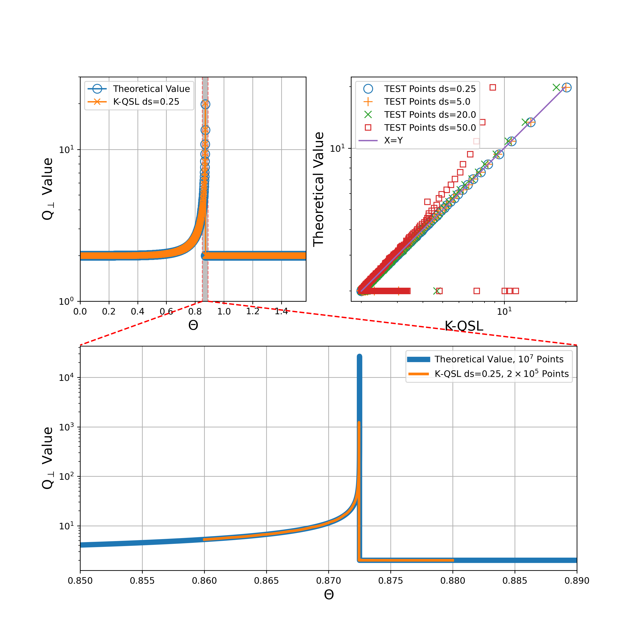
The upper-left panel reveals a close match between K-QSL results and theoretical values. Along the latitude,
- non-uniform magnetic field (progress ... 100%).
- adaptive mesh refinement for capturing the fine structure (progress ... 90%).
- A new method will come soon (progress ... 50%).